What did peak union power look like on the ground in human terms? Decades of scholarship, still evolving, gives us a nuanced sense of local struggles linked to national and international issues. But it is sometimes harder to get a holistic sense of the movement, to see the linkages across organizations and campaigns. How were labor’s “strategic actors” distributed across the landscape of industrial society? Was the organizational terrain full of links between groups and people of different backgrounds, or barriers separating activists?
We can get some preliminary answers by mapping the 1946 Who’s Who in Labor. The directory contains nearly 4,000 entries, and like earlier directories has certain limitations. Labor union officials in 1946 were disproportionately male and predominately Euro-American. Unlike the directors of the mid-1920s that encompassed a “labor movement” of unions, political parties, and cooperatives, the postwar version sticks pretty close to the union movement itself. On the plus side, the labor movement of 1946 was yet to be ravaged by the Cold War anticommunist crusades. Still in the ranks were left-led unions that would be expelled in 1949. Leadership of unions like the UE, FE, FTA, Mine Mill, United Public Workers, and the Furriers.
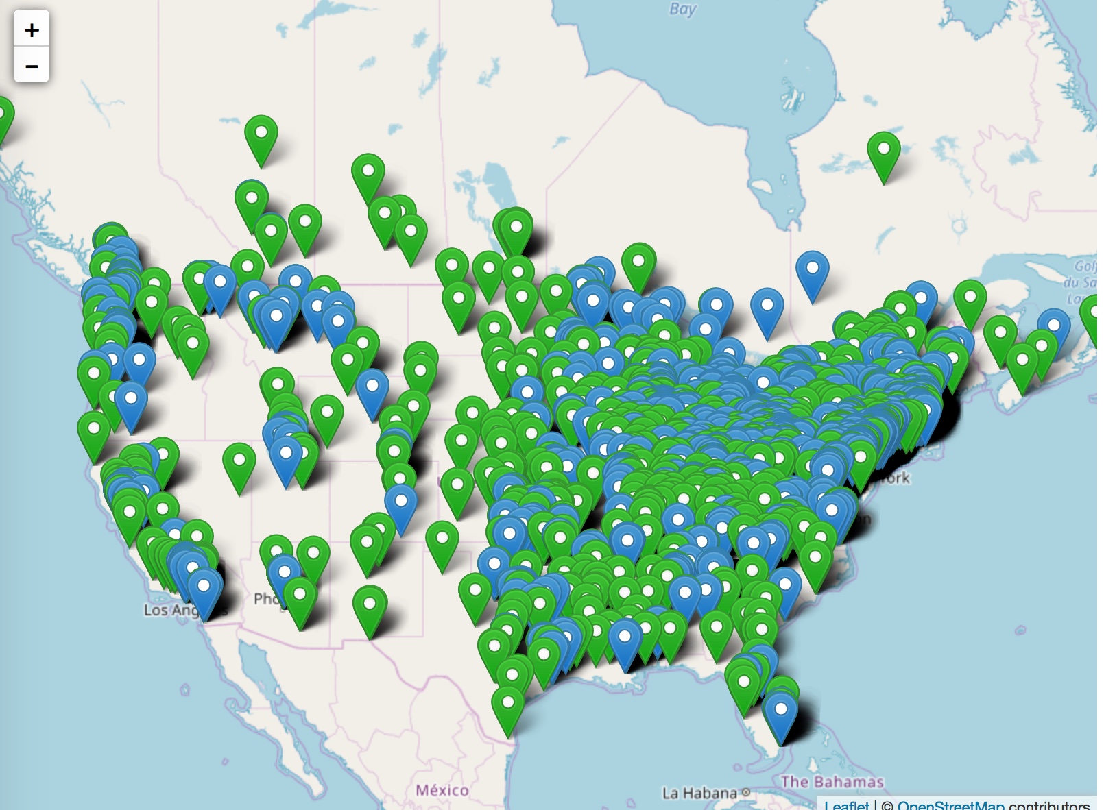
Over the next few months I will be refining this data set, but for now I offer a spatial comparison between members of the AFL and the CIO. (If the embedded map doesn’t resolve, try this link: AFL and CIO Leaders, 1946 with AFL in Green and CIO in blue). A few initial thoughts on this map. First, while union leaders are pretty dense across the Midwest and Northeast, one can clearly see the clustering of CIO leaders in larger cities, and the spread of AFL leaders across the less densely populated areas. Manhattan, for instance, is densely packed with union officials–not surprising, but visually striking. Across the South, there are relatively more AFL leaders with the exception of Birmingham and Atlanta.
For now, you have to click on each marker to get information beyond the AFL/CIO distinction. The maps is likely most interesting at the city level where, especially if you know the city and/or its labor history, you can see which leaders lived nearby each other, trace the racial boundaries of neighborhoods, and get a sense of how much influence unions likely had on municipal politics. In the future we’ll add filtering and searching. More to come. Raw data on Github.
Process Notes
In the past, I’ve worked with GoogleMaps and Carto. My colleague Jim Gregory makes extensive use of Tableau to distribute maps and charts from his Mapping American Social Movements project. These commercial packages make it easy to display maps and data, but I am eager to make use of open source platforms. My goal is to keep the data as simple as possible (CSV files) to avoid having the data trapped in a proprietary platform. I am also curious to see whether a person with modest technical background can use these open source platforms and tools. This new batch of data gave me the opportunity to try my hand at Leaflet, an opensource java script library for making online maps.
I turned to the always-helpful site Programming Historian for a lesson on Mapping with Python and Leaflet. I was able to get about half way there on my own, and then got a crucial assist from the staff in our departmental computer support office. You need to learn a bit of Python code so you can run the geocoding program, and in the process you will learn a little about Leaflet. If you can follow instructions, have a modest capacity for troubleshooting, and know some computer science students, then you can do this. Whether you plan to go deeper into these programs or hand it off to an expert, I think it’s probably worth spending a little time understanding the basic concepts behind web mapping.